Remember in machine learning courses, you learn that AUC is a useful metric to evaluate classifier. The higher the value (ranges from 0 to 1), the better the model is. However, what exactly is AUC and what makes it a great metric? We’ll have a deep dive and explore the theory behind.

AUC - Area Under ROC Curve

AUC is short for the Area Under ROC (Receiver Operating Characteristics) curve. As a general performance metric, AUC measures the binary classification model performance without the need to specify a threshold. Note that AUC could only be calculated if the model is capable of providing probability prediction. Before going further into AUC, let’s first talk about the ROC curve.

ROC Curve - Receiver Operating Characteristics Curve

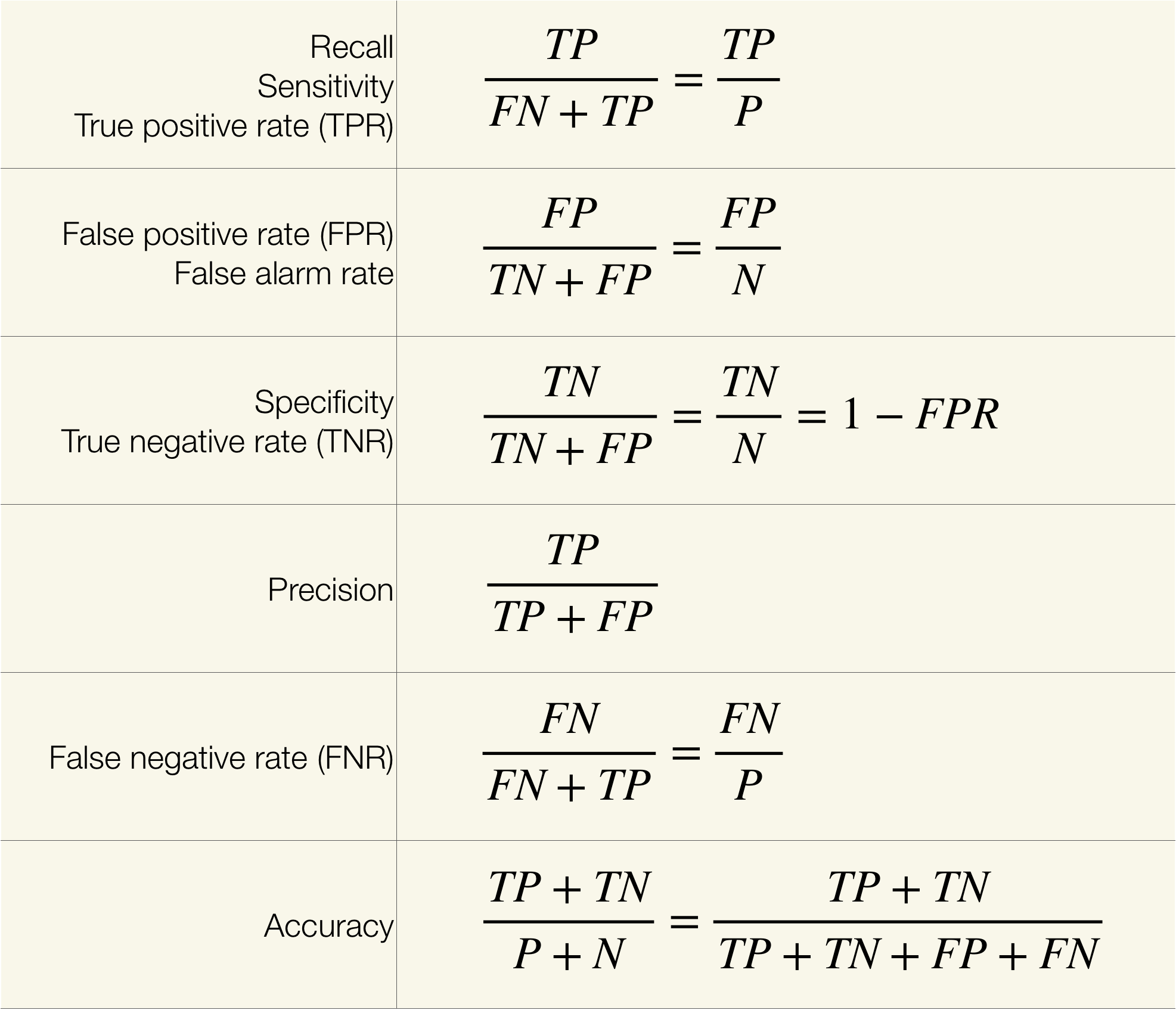
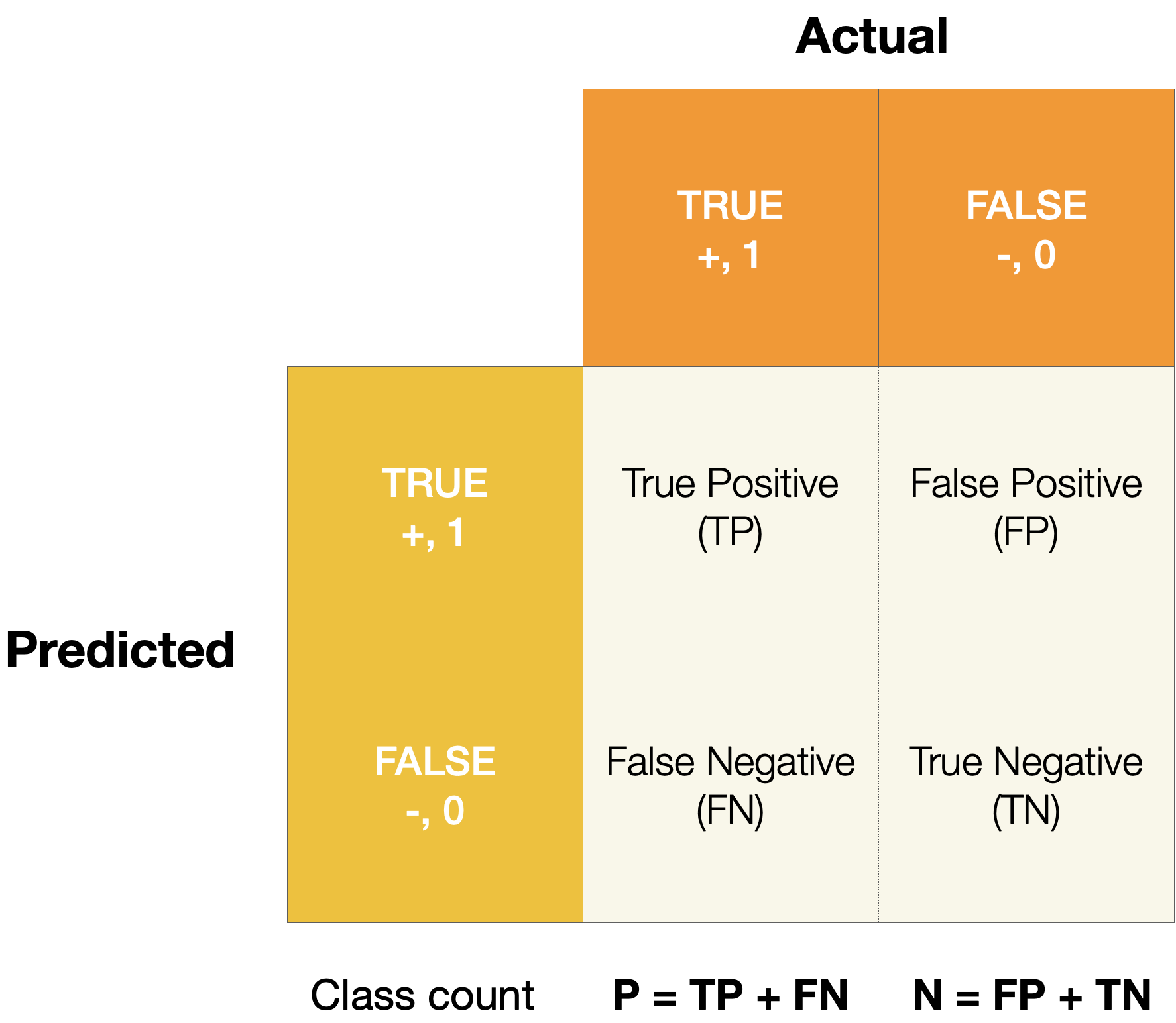
In the figure below, the confusion matrix summarizes all of the possible conditions - true positive, false positive, true negative and false negative of a binary classification model. False positive and false negative indicate that the model incorrectly identifies the case, whereas true positive and true negative show the predictions are correct. One thing to note here is that all the measurements are determined by the predicted classes based on individual cut-off threshold of the probability. In other words, all of the measurements are single-threshold measures and they cannot provide an overview of the performance with varying threshold.

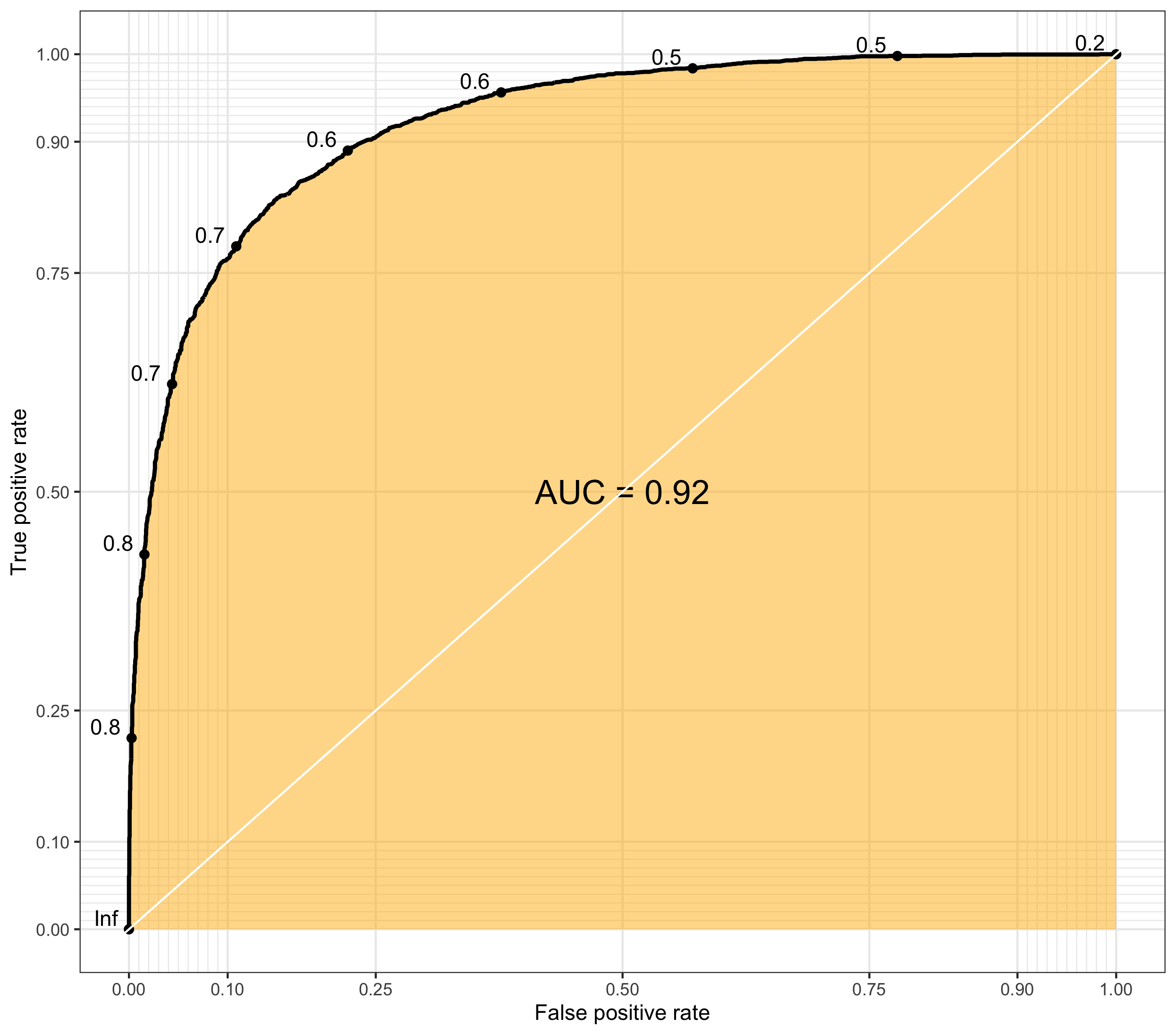
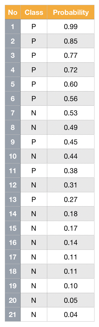
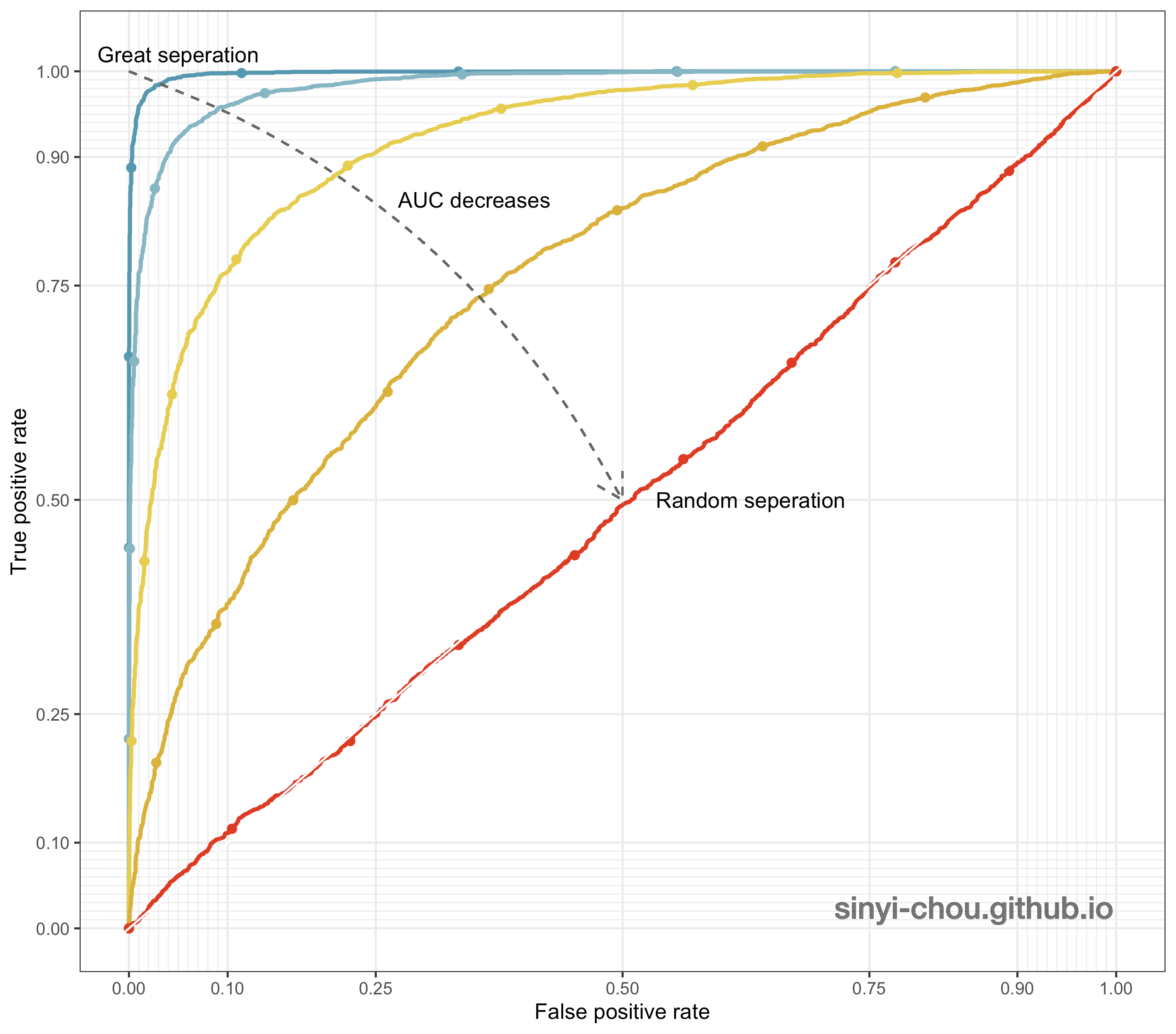
Threshold-invariant metrics, such as AUC & logloss, are capable of measuring the overall model performance despite any chosen threshold. The figure below is a plot of ROC curve, in which false positive rate - FPR (x-axis) and true positive rate - TPR, or also called recall, (y-axis) are used for plotting. Each point in the ROC curve is computed based on the specific cutoff threshold that is labeled on the plot, and AUC is the area under the curve - the yellow area. While the ROC curve moves towards the upper-left corner, the value of AUC increases with higher TPR and lower FPR for any threshold.

Below animation illustrates the outcome when different cut-off thresholds are chosen. FPR starts off at 0 with a high threshold. When the threshold decreases, TPR and FPR would both increase with more false positive being classified and more true positive found. TPR would eventually reach 1 until all of the positive classes are identified correctly. If the goal is to find all of the positive instances correctly, higher TPR/recall is favored. In contrast, smaller FPR is favored when the interest is to find all of the negative instances correctly. In short, TPR:1 and FPR:0 is the desired conditions.

The optimal threshold is normally chosen based on domain knowledge and applications, thus no single criteria can be used to determine the optimal threshold of a classifier. Namely, cancer prediction models would have a threshold quite different from that of credit card approval prediction models. Cancer models aim to identify as many potential patients as possible even if some patients are falsely identified, whereas credit card approval models aims to identify the most qualified applicants in order to minimize false positives rate. Other measures, such as F1-measure, are also often used to determine the optimal threshold. F1-measure is capable of managing the trade off between precision and recall rate to determine a balanced performance.

Probabilistic Interpretation of AUC

In the probabilistic perspective, AUC is the probability of a randomly chosen positive case outranks a randomly chosen negative case based on the classifier.

$$AUC = P(f(x+) > f(x-)|class(x+)=1, class(x-)=0)\\ = \frac{1}{PN}\sum_{i=1}^{P}\sum_{j=1}^{N} 1(f(x+)-f(x-))\\ f(x) : classifier $$ P : # of true positive item, N : # of true negative item

In other words, it measures how well the probability ranks based on their true classes. Thus, it is a threshold-invariant and scale-invariant metrics and only the sequence matters in the predicted probabilities. Based on this property, models with higher AUC indicate better discrimination between the two classes. However, the probabilities output from models with higher AUC don’t always generate well-calibrated probabilities. More information can be found here: Safe Handling Instructions for Probabilistic Classification.

In a real life application, finding a focused group for marketing campaign targeting is a good example for using AUC since the relative probability of each instance (rank) is of interest instead of absolute probability

Visualization

To visualize how AUC is affected by different level of separation/discrimination, the distribution of probability for both the positive and negative classes are plotted below. When the overlap of two classes increases, the harder it gets to separate them and results in the decrease of AUC - random separation, at which AUC is equal to 0.5. Interestingly, the classifier can be a good one after reversing the predictions if the ROC curve lies in the right-bottom corner with AUC <=0.5.

Summary

1. AUC is a threshold-free metrics capable of measuring the overall performance of binary classifier.

2. AUC can only be used in binary classification. In multinomial classification, one-to-rest AUC would be an option using the average of each class.

3. AUC is a good metric when the rank of output probabilities is of interest.

4. Although AUC is powerful, it is not a cure-all. AUC is not suitable for heavily imbalanced class distribution and when the goal is to have well-calibrated probabilities.

5. Models with maximized AUC treat the weight between positive and negative class equally.

Reference

1. An introduction to ROC analysis
2. Google Machine Learning Crash Course
3. ROC Curve
4. ROC curves and Area Under the Curve explained
5. AUC Visualization
6. Probabilistic interpretation of AUC

All the plots and animation in this post are made on my own with ideas inspired by above references. Please reference my website when used.